STAT 250 Fall 2020 Data Analysis Assignment

Your submitted document should include the following items.  Points will be deducted if the following are not included.

1. Type your Name and STAT 250 with your correct section number (e.g. STAT 250-xxx) right justified and then Data Analysis Assignment #2 centered on the top of page 1 below your name the begin your document.
2. Number your pages across your entire solutions document.
3. Your document should include the ANSWERS ONLY with each answer labeled by its corresponding number and subpart. Keep the answers in order. Do not include the questions in your submitted document.
4. Generate all requested graphs and tables using StatCrunch.
5. Upload your document onto Blackboard as a Word (docx) file or pdf file using the link provided by your instructor.  It is your responsibility for uploading a readable file.
6. You may not work with other individuals on this assignment.  It is an honor code violation if you do.

Elements of good technical writing:

Use complete and coherent sentences to answer the questions.

Graphs must be appropriately titled and should refer to the context of the question.

Graphical displays must include labels with units if appropriate for each axis.

Units should always be included when referring to numerical values.

When making a comparison you must use comparative language, such as “greater than”, “less than”, or “about the same as.”

Ensure that all graphs and tables appear on one page and are not split across two pages.

Type all mathematical calculations when directed to compute an answer ‘by-hand.’

Pictures of actual handwritten work are not accepted on this assignment.

When writing mathematical expressions into your document you may use either an equation editor or common shortcuts such as:  can be written as sqrt(x), can be written as p-hat, can be written as x-bar.

Problem 1: Simulating Rolling Two Four-Sided Dice (no data set)

We will be comparing empirical (relative frequencies based on an observation of a real-life process) to theoretical (long-run relative frequency) probabilities.  We will use StatCrunch to simulate rolling two four-sided dice.  Conduct the following simulation by using the steps below:

1. Step 1: Under Applets à Simulation à Select Dice rolling from the menu.

Step 2: In window, enter 4 for the number of sides and 2 for the number of dice.  (edit)

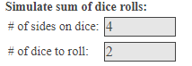
Step 3: Select Compute!

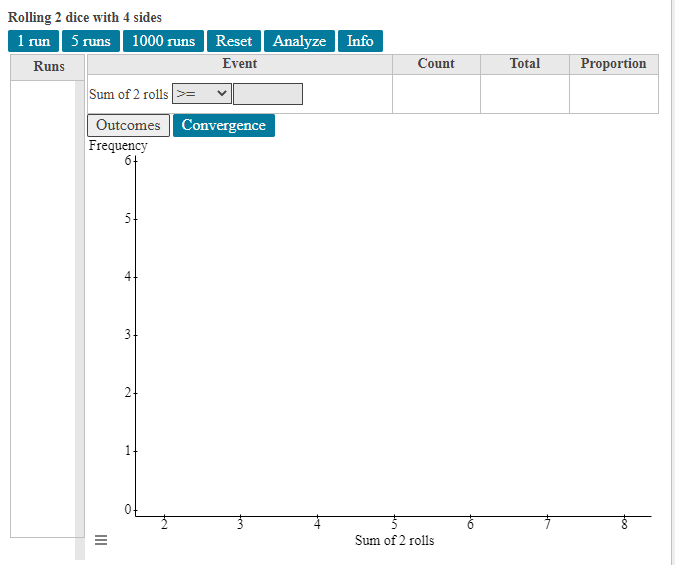
Step 4: Select 1000 runs to simulate rolling the two dice 1000 times as shown below. The result of this simulation will appear as a bar graph.

Step 5: Clear the box to the right of “Sum of 2 rolls” for part (a) (none of the bars in the chart will now be highlighted).

Step 6: Copy your chart into your document for your answer to part (a).

 NOTE: You will use this result to answer parts (c) – (h).

 

Using your result from the 1000-run simulation found in part (a), find the following three  proportions for parts (c) – (h) and then compare these empirical probabilities with their theoretical probabilities. DO NOT GENERATE ANOTHER RESULT. You only need to adjust the information in boxes 1 and 2 above to answer parts (c) – (h).  Please complete parts (c) – (h) in one sitting so you use the same simulation results.

1. Build the probability distribution for the sum of two four-sided dice (i.e. list the possible values of the random variable, X (sum of two four-sided dice) and each value’s corresponding probability) in table form and present this table in your document. Use the x-axis above and rules of theoretical probability to calculate your probabilities.  Present the probabilities as fractions or decimals in the table.  Note, you can use this table to calculate your theoretical probabilities in parts (c) – (h).
2. Under Event in the applet, enter: “Sum of 2 rolls equals 7.” Use options à copy to copy this chart into your document.
3. Now calculate the theoretical probability that “Sum of 2 rolls equals 7” using the sample space or the probability distribution built in part (b). State this probability as a decimal rounded to three decimal places in a sentence.
4. In another sentence, compare your empirical probability (found in the simulation) to the theoretical probability of obtaining a sum of 2 rolls equal to 7. Remember to justify your answer by including the values.
5. Under Event now find: “Sum of 2 rolls greater than or equal to 7.” Use options à copy to copy this chart into your document.
6. Now calculate the theoretical probability that “Sum of 2 rolls greater than or equal to 7” using the sample space or the probability distribution built in part (b). State this probability as a decimal to rounded to three decimal places in a sentence.
7. In another sentence, compare the empirical probability (found in the simulation) to the theoretical probability of obtaining a sum of two rolls that is greater than or equal to 7.
8. Under Event find: “Sum of 2 rolls less than 7” Use options àcopy to copy your answer into your document.
9. Now calculate the theoretical probability that “Sum of 2 rolls less than 7” using the sample space or the probability distribution built in part (b).  State this probability as a decimal rounded to three decimal places in a sentence.
10. In another sentence, compare the empirical probability (found in the simulation) to the theoretical probability of obtaining a sum of two rolls that is less than 7.

Problem 2: VW Bus Auction Sales

The Volkswagen Type 2, informally known as the VW Bus, was first introduced in 1950.  The first generation of the Type 2, which was produced until 1967, has an active aftermarket with vehicles frequently sold for high prices at auction.  The dataset (called “VW Bus Auction Sales”) for the winning bid of 126 unrestored VW Type 2’s sold at auction are given on StatCrunch.

1. Use StatCrunch to construct an appropriately titled and labeled relative frequency histogram of the winning bid (in dollars). Copy your histogram into your document.
2. What is the shape of this distribution? Answer this question in one complete sentence.
3. Using your histogram, determine the proportion of winning bids of $75,000 or more. To do this, click on each bar that is representing $75,000 or more and look in the bottom left to see how many individual times are highlighted.  Provide the image of the highlighted histogram and the correct proportion (type your work for the calculation of the proportion).
4. Now overlay your highlighted histogram from 2(c) with a normal curve and add a vertical line at the mean.

This can be done by going to Options à Edit in the top left corner of your graph.  Inside the histogram graph box, look for Display Options.  Next to “Overlay distrib.:” click the arrow next to the word –optional– and select Normal.  Then, check the box next to mean under the word “Markers.” Copy and paste this histogram into your document.

1. Do you think it is reasonable to use the normal probability model in this case? Answer this question and provide a reason why in one sentence.
2. Calculate the sample size, the mean, and the standard deviation of the “Winning Bid” variable using StatCrunch. (Select Stat à Summary Stats à)  Copy and paste this table into your document.  Round the mean and standard deviation to whole numbers inside this table.

For parts (g) – (l), assume that the distribution of winning bid prices in the population is normal with the mean and standard deviation found in part 2(f) (again use the rounded mean and standard deviation values).  Note: you are using the normal distribution for the next three calculations.

1. Calculate the probability that a randomly selected winning bid is $75,000 or more. First, draw a picture with the mean labeled and shade the area representing the desired probability.  Next, standardize the value and use the Standard Normal Table (Table 2 in your text) to obtain this probability.  Then, take a picture of your hand drawn sketch and upload it to your document (if you do not have this technology, you may use any other method (i.e. Microsoft paint) to sketch the image into your document).  You must type the rest of your “by hand” work to earn full credit.
2. Verify your answer in part (g) using the StatCrunch Normal calculator and copy that image with the values displayed into your document. In addition, write one sentence to explain what the probability means in context of the question.
3. Compare this probability to the proportion you calculated in part (c). Label each probability as a theoretical or an empirical probability in your comparison.
4. Use StatCrunch only to calculate the probability that a randomly selected winning bid is between $55,300 and $67,200. Copy the normal distribution image from StatCrunch with the values displayed into your document.  Then, once you obtain your answer, write one sentence to explain what the probability means in context of the question.
5. An individual looking to obtain a VW Bus is looking for a good deal. They will only place a bid on the bus if it is within the 7.5^th percentile (i.e. the bottom 7.5%) of all winning bids.  What is the maximum value that this individual is willing to bid?  Draw a picture of the density curve, shade the area, and use the standard normal table to solve this problem.  Take a picture of your hand drawn sketch and upload it to your document (if you do not have this technology, you may use any other method (i.e. Microsoft paint) to sketch the image).  You must type the rest of your “by hand” work to earn full credit.
6. Verify your answer in part (k) using the StatCrunch Normal calculator and copy that image into your document. In addition, write one sentence to explain what the probability means in context of the question.

Problem 3: GMU Student Voting Percentage (no data set)

A Mason Votes article published on November 14^th, 2019 shares a table for the George Mason registration and voting rates from the 2012 to 2018 Presidential and Midterm Elections from data submitted and collected by National Student Clearinghouse and Catalist. The voting rate for all students, registered and non-registered, in the 2016 Presidential Election was 64.9%. A random sample of 15 students from GMU in Fall 2016 were selected and asked the question, “Did you vote in the 2016 Presidential Election?”

Mason Votes is a fantastic resource that provides information and guides individuals regarding registration, upcoming events, and other election news specific to George Mason University.  Find more info at: http://masonvotes.gmu.edu/.

1. Check if this situation fits the binomial setting. Write four complete sentences addressing each requirement. Use one sentence for each requirement
2. Assuming this situation is a binomial experiment, build the probability distribution in a single table form in StatCrunch. There are two ways to do this.  You may use Data à Compute à Expression and choose the function dbinom.  This method relies on you entering all the outcome values of the random variable in the first column of your data table.  The other way to do this is to use the binomial calculator and calculate the probability of each of the values of the random variable from X = 0 to X = 15.  You may present this table horizontally or vertically and leave the probabilities unrounded.
3. Calculate the probability that more than half of the 15 students, at least 8, in this sample voted in the 2016 Presidential Election using the probability distribution table you created in 3(b). Show all of your calculations and use proper probability notation. You do not need to round your answer or the probabilities.
4. Verify your answer to 3(c) using the StatCrunch binomial calculator. Copy the image with values below to your document. Write a one sentence interpretation of the probability in context of the question.
5. Calculate the probability that between seven and eleven (inclusive) of the students in this sample voted during the 2016 Presidential Election using the StatCrunch binomial calculator graph and include this image with values in your document. Write a one sentence interpretation of the probability in context of the question.
6. What is the average number of students in the sample do you expect to respond “yes” to voting in the 2016 President Election? To answer this question, calculate the mean and standard deviation of this probability distribution.  Show your work using the binomial mean and binomial standard deviation formulas and provide your answers in your document.  Round your answers to two decimal places. (It is not necessary to use StatCrunch for this part).
7. Calculate the probability that exactly ten of the 15 students in this sample voted during the 2016 Presidential Election using the StatCrunch binomial calculator. Copy this image with values from StatCrunch into your document.  Then, once you obtain your answer, write a one sentence interpretation of the probability in context of the question.
8. Imagine you repeated taking a sample of 15 students from the GMU population 10,000 times. We can simulate this in StatCrunch.  First, go to Data à Simulate à  Next, enter 10,000 for Rows, 1 for Columns, 15 for n, 0.649 for p, and click compute.  Then, to visualize these data, go to Graph à Bar Plot à With Data.  Produce a properly titled and labeled relative frequency bar plot and paste it into your solutions.
9. State the height of the bar above ten and compare this with your answer to part 3(g). Identify which type of probability each value is in your comparison.

Problem 4 on the next page.

Problem 4: Building a Sampling Distribution (no data set)

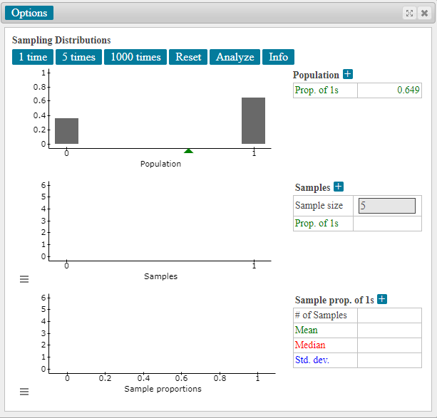
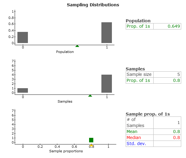
We will use the Sampling Distribution applet in StatCrunch to investigate properties of the sampling distribution of the proportion of students at GMU who voted in the 2016 Presidential Election from the previous problem.  Remember, the given probability of students at Mason who voted in the 2016 Presidential Election is 0.649.  We will begin by taking a sample of 5.

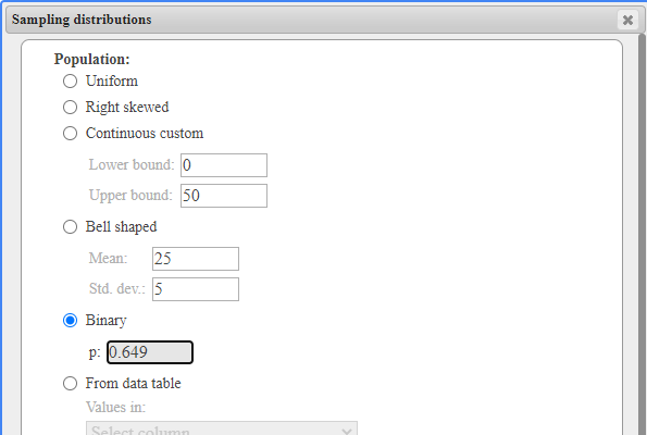
Under Applets, open the Sampling distribution applet (box shown below).  First, select Binary for the population.  Next, to the right of “p:”, enter 0.649 which is the probability of a student at GMU who voted in the 2016 Presidential Election.  Then click on Compute!  See image below.

 

1. Once the applet box is opened, enter 5 in the box to the right of the words “sample size” in the right middle of the applet box window (see image below). Then, at the top of the applet, click “1 time.”  Watch the resulting animation.  When the sample is completed, copy and paste the entire applet box (using options à copy) into your document.

1. Click “Reset” at the top of the applet. Then, click the “1000 times” to take 1000 samples of size 5.  Copy and paste the applet image into your document.
2. Describe the shape of the Sample Proportions graph at the bottom of your image from part 4(b) in one sentence.
3. Use the Central Limit Theorem large sample size condition to determine if it is reasonable to define this sampling distribution as normal. Explicitly show these calculations for the condition in your answer. Write a one sentence explanation on the condition and the calculations.
4. Click Reset at the top of the applet. Type 100 in the sample size box.  Then, click the “1000 times” to take 1000 samples of size 100.  Copy and paste the applet image into your document.
5. Describe the shape of the Sample Proportions graph at the bottom of your image from part 4(e) in one sentence.
6. Why do you think that this graph from part 4(e) has the shape you described? Use the Central Limit Theorem large sample size condition to answer this question in one sentence.  Explicitly show these calculations for the condition in your answer. Write a one sentence explanation on the condition and the calculations.
7. Using the image in part 4(e), write the values you obtained for the mean (in green) and the standard deviation (in blue). These values are found in the bottom right box labeled “Sample Prop. of 1s.”
8. Compare the mean value (in green, found in part 4(h)) to the known population proportion in one sentence. Make sure to reference the values in your comparison.
9. Now calculate the standard error of the sample proportion using p = 0.649 and n = 100 by hand. Type your “by hand” work for the calculations and round your answer to four decimal places.
10. Compare the value in part 4(j) to the standard deviation (in blue) you obtained in part 4(h) in one sentence. Make sure to reference the values in your comparison
11. Use the sampling distribution defined by the Central Limit Theorem to calculate the probability that from a sample of 100 students at least 76% of students that were registered in 2016 at George Mason University would have voted in the Presidential Election of that year (use p = 0.649 and the standard error found in part 4(j)).

 

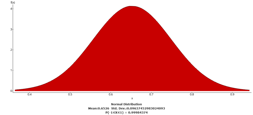
First, draw a picture with the mean labeled and shade the area representing the desired probability.  Next, standardize using the proper calculations and use the Standard Normal Table (Table 2 in your text and formula sheet) to obtain this probability.  Then, take a picture of your hand drawn sketch and upload it to your document (if you do not have this technology, you may use any other method (i.e. Microsoft paint) to sketch the image).  You must type the rest of your “by hand” work (e.g. the formula and calculations used to find the z-value) to earn full credit.

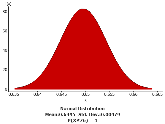
Provide a StatCrunch Normal graph to verify the work in part 4(l) and write one complete sentence to interpret the resulting probability in context of the question.

HINT: Remember to use the values you used in 4(l).

 

ANSWER

 

Problem 1: Simulating Rolling Two Four-Sided Dice (no data set)

Chart

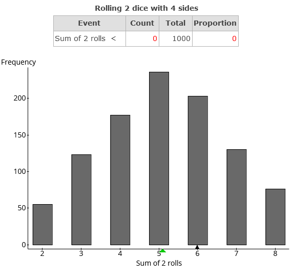
Table and Graph

 

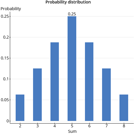
Sum of rolls	Probability
2	0.0625
3	0.125
4	0.1875
5	0.25
6	0.1875
7	0.125
8	0.0625
	1

 

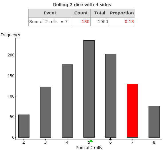
Graph, sum of 2 rolls is 7

Theoretic vs empirical probability

The theoretic probability of the Sum of two rolls equals to 7 is 0.125

The empirical probability of the Sum of two rolls equals to 7 is 0.130. This difference is because the first is a hypothetical result while the second is an actual experimental result

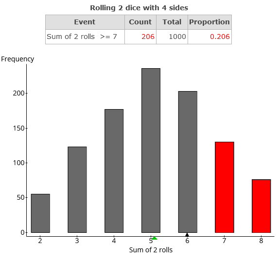
Graph – Sum of two rolls is equal to or greater than 7

Theoretic vs empirical probability

The theoretic probability of the sum of two rolls equals to or greater than 7 is 0.1875

The empirical probability of the sum of two rolls equals to or greater than 7 is 0.206. This difference is because the first is a hypothetical result while the second is an actual experimental result

Graph- sum of two rolls is less than 7

 

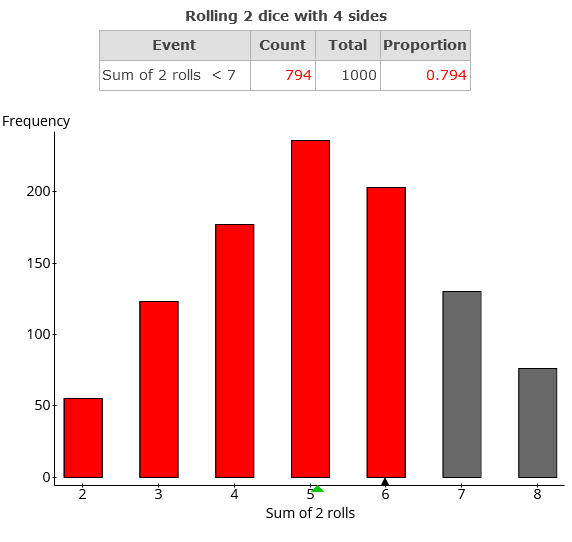
Theoretic vs empirical probability

The theoretic probability of the sum of two rolls is less than 7 is 0.8125

The empirical probability of the sum of two rolls is less than 7 is 0.794. This difference is because the first is a hypothetical result while the second is an actual experimental result

Problem 2: VW Bus Auction Sales

Histogram of winning bid

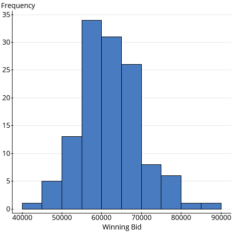
Distribution shape

The shape of the distribution is bell shaped which suggests it is a normal distribution

Proportion above 75,000

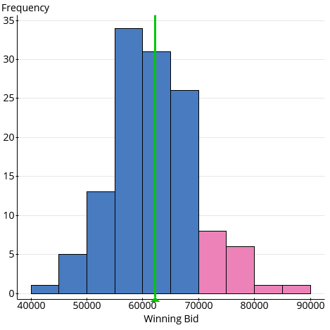
8 bids between $75,000 and $90,000

Overlay

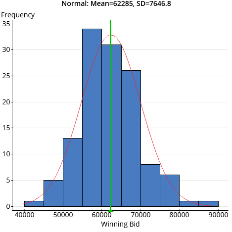
Normal probability model

It is okay to use a normal probability model in this case because the shape of the distribution, the mean and standard deviation give it the distinctive shape.

Summary statistics

Column	n	Mean	Std. dev.
Winning Bid	126	62285.222	7646.7843

 

Hand drawing

Client to do this using own hand. Draw diagram below

Verification

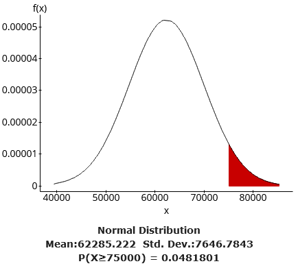
Compare this probability to the proportion

The probability and the proportion are almost equal with one being the theoretical and the other being the experimental probability

Probability diagram

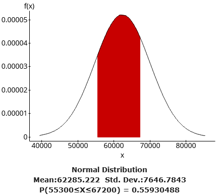
Hand diagram

Verification

Problem 3: GMU Student Voting Percentage (no data set)

Binomial experiment requirements

A binomial experiment must have n identical trials.

Each of these n trials must be independent

Each trial only has two possible outcomes e.g. Yes/ No, Success/ Failure, etc.

The probability of an outcome remains the same in each trial

Using the binomial calculator to produce probability distribution

x	p(x,n,p)
0	0.00000015
1	0.00000419
2	0.00005428
3	0.00043494
4	0.00241262
5	0.00981409
6	0.0302438
7	0.07189826
8	0.13294008
9	0.1911829
10	0.21209864
11	0.17825954
12	0.10986747
13	0.04687967
14	0.01238295
15	0.00152641
	0.99999999

 

Example

At least eight voted P (8, 15, 0.649) manual calculation

x	p(x,n,p)
0	0.00000015
1	0.00000419
2	0.00005428
3	0.00043494
4	0.00241262
5	0.00981409
6	0.0302438
7	0.07189826
8	0.13294008
	0.24780241

 

P (8, 15, 0.649) = 0.24780241

At least eight voted P (8, 15, 0.649) StatCrunch calculation

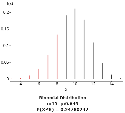
P (8, 15, 0.649) = 0.24780242

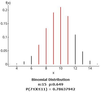
Between 7 and 11 voted P (7≤X≤11, 15, 0.649) StatCrunch calculation

This is the probability of between 7 to 11 students voting, excluding less than 7 and more than 11.

Mean and SD

Mean of the distribution (μx) is n * P i.e. 15*0.649 = 9.735

Standard deviation (σx) is sqrt [n * P * (1 – P)] i.e. sqrt [9.735*0.351] = 1.849

Exactly 10 voted, StatCrunch calculation

 

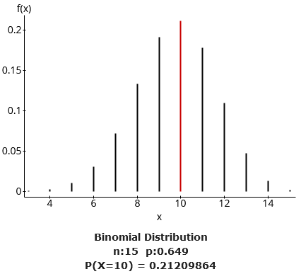
P (10, 15, 0.649) = 0.21209864

Relative frequency bar plot

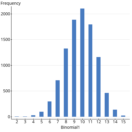
Height of bar above ten is 2104. Compared to part 3(g) where the probability was 0.21209864, the expected result would have been 2120. But the latter is a theoretical probability while the former is empirical

Problem 4: Building a Sampling Distribution (no data set)

Sampling distribution

 

1000 samples of size 5

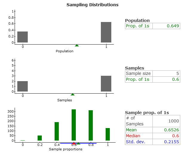
Shape of the Sample Proportions graph

The sample has a bell shaped curve which suggests it’s a normal distribution

Central Limit Theorem

Sample size 100 for 1000 trials

 

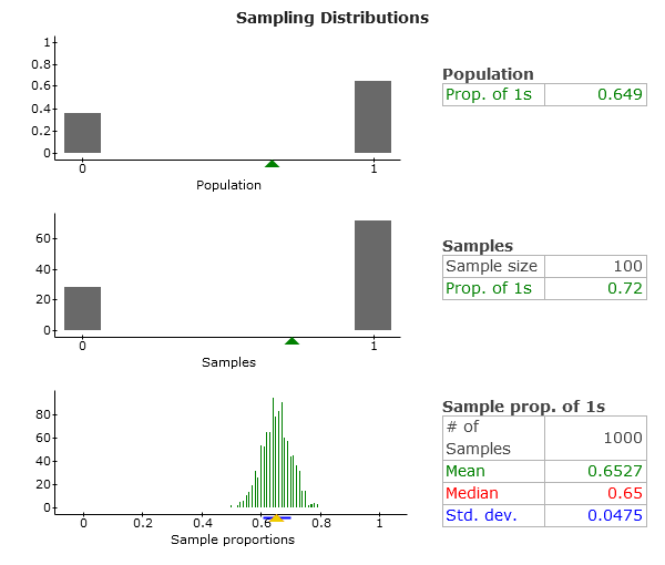
Graph description

The sample has a bell shaped curve which suggests it’s a normal distribution

Central Limit Theorem

 

Mean – 0.6495

SD – 0.0479

Mean value vs population proportion.

The mean mimics the value proportion of the population of 100 in the sample

Standard error

SE = SD/sqrt(n) i.e. 0.0479/sqrt (100) = 0.00479

Standard error vs SD

The standard error is simply the standard deviation divided by 10 or a tenth

 Hand diagram

Copy diagram below by hand

 

To get your original copy of this completed paper, please Order Now